1.2.6. Tutorials

This chapter walks users through experiment configuration options for various severe weather events. It assumes that users have already built the SRW App successfully.

Users can run through the entire set of tutorials or jump to the one that interests them most. The first tutorial is recommended for users who have never run the SRW App before. The five tutorials address different skills:

1. Severe Weather Over Indianapolis: Change physics suites and compare graphics plots.

2. Cold Air Damming: Coming soon!

3. Southern Plains Winter Weather Event: Coming soon!

4. Halloween Storm: Coming soon!

5. Hurricane Barry: Coming soon!

Each section provides a summary of the weather event and instructions for configuring an experiment.

1.2.6.1. Sample Forecast #1: Severe Weather Over Indianapolis

Objective: Modify physics options and compare forecast outputs for similar experiments using the graphics plotting task.

1.2.6.1.1. Weather Summary

A surface boundary associated with a vorticity maximum over the northern Great Plains moved into an unstable environment over Indianapolis, which led to the development of isolated severe thunderstorms before it congealed into a convective line. The moist air remained over the southern half of the area on the following day. The combination of moist air with daily surface heating resulted in isolated thunderstorms that produced small hail.

Weather Phenomena: Numerous tornado and wind reports (6/15) and hail reports (6/16)

• Storm Prediction Center (SPC) Storm Report for 20190615

• Storm Prediction Center (SPC) Storm Report for 20190616

Fig. 1.5 Severe Weather Over Indianapolis Starting at 18z

1.2.6.1.2. Data

On Level 1 systems, users can find data for the Indianapolis Severe Weather Forecast in the usual input model data locations (see Section 1.10 for a list). The data can also be downloaded from the UFS SRW Application Data Bucket.

• FV3GFS data for the first forecast (control) is located at:

  • https://noaa-ufs-srw-pds.s3.amazonaws.com/index.html#input_model_data/FV3GFS/grib2/2019061518/

• HRRR and RAP data for the second forecast (test_expt) is located at:

  • https://noaa-ufs-srw-pds.s3.amazonaws.com/index.html#input_model_data/HRRR/2019061518/

  • https://noaa-ufs-srw-pds.s3.amazonaws.com/index.html#input_model_data/RAP/2019061518/

1.2.6.1.3. Load the Workflow

To load the workflow environment, source the lmod-setup file. Then load the workflow conda environment. From the ufs-srweather-app directory, run:

source etc/lmod-setup.sh <platform>       # OR: source etc/lmod-setup.csh <platform> when running in a csh/tcsh shell
module use modulefiles
module load wflow_<platform>

where <platform> is a valid, lowercased machine name (see MACHINE in Section 1.3.1.1 for valid values).

After loading the workflow, users should follow the instructions printed to the console. Usually, the instructions will tell the user to run conda activate srw_app. For example, a user on Hera with permissions on the nems project may issue the following commands to load the workflow (replacing User.Name with their actual username):

source /scratch1/NCEPDEV/nems/User.Name/ufs-srweather-app/etc/lmod-setup.sh hera
module use /scratch1/NCEPDEV/nems/User.Name/ufs-srweather-app/modulefiles
module load wflow_hera
conda activate srw_app

1.2.6.1.4. Configuration

Navigate to the ufs-srweather-app/ush directory. The default (or “control”) configuration for this experiment is based on the config.community.yaml file in that directory. Users can copy this file into config.yaml if they have not already done so:

cd /path/to/ufs-srweather-app/ush
cp config.community.yaml config.yaml

Users can save the location of the ush directory in an environment variable ($USH). This makes it easier to navigate between directories later. For example:

export USH=/path/to/ufs-srweather-app/ush

Users should substitute /path/to/ufs-srweather-app/ush with the actual path on their system. As long as a user remains logged into their system, they can run cd $USH, and it will take them to the ush directory. The variable will need to be reset for each login session.

1.2.6.1.4.1. Experiment 1: Control

Edit the configuration file (config.yaml) to include the variables and values in the sample configuration excerpts below.

Hint

To open the configuration file in the command line, users may run the command:

vi config.yaml

To modify the file, hit the i key and then make any changes required. To close and save, hit the esc key and type :wq to write the changes to the file and exit/quit the file. Users may opt to use their preferred code editor instead.

Start in the user: section and change the MACHINE and ACCOUNT variables. For example, when running on a personal MacOS device, users might set:

user:
   RUN_ENVIR: community
   MACHINE: macos
   ACCOUNT: none

For a detailed description of these variables, see Section 1.3.1.1.

Users do not need to change the platform: section of the configuration file for this tutorial. The default parameters in the platform: section pertain to METplus verification, which is not addressed here. For more information on verification, see Section 1.2.7.

In the workflow: section of config.yaml, update EXPT_SUBDIR and PREDEF_GRID_NAME.

workflow:
  USE_CRON_TO_RELAUNCH: false
  EXPT_SUBDIR: control
  CCPP_PHYS_SUITE: FV3_GFS_v16
  PREDEF_GRID_NAME: SUBCONUS_Ind_3km
  DATE_FIRST_CYCL: '2019061518'
  DATE_LAST_CYCL: '2019061518'
  FCST_LEN_HRS: 12
  PREEXISTING_DIR_METHOD: rename
  VERBOSE: true
  COMPILER: intel

Note

Users may also want to set USE_CRON_TO_RELAUNCH: true and add CRON_RELAUNCH_INTVL_MNTS: 3. This will automate submission of workflow tasks when running the experiment. However, not all systems have cron.

EXPT_SUBDIR: This variable can be changed to any name the user wants from “gfsv16_physics_fcst” to “forecast1” to “a;skdfj”. However, the best names will indicate useful information about the experiment. This tutorial uses control to establish a baseline, or “control”, forecast. Since this tutorial helps users to compare the output from two different forecasts — one that uses the FV3_GFS_v16 physics suite and one that uses the FV3_RRFS_v1beta physics suite — “gfsv16_physics_fcst” could be a good alternative directory name.

PREDEF_GRID_NAME: This experiment uses the SUBCONUS_Ind_3km grid, rather than the default RRFS_CONUS_25km grid. The SUBCONUS_Ind_3km grid is a high-resolution grid (with grid cell size of approximately 3km) that covers a small area of the U.S. centered over Indianapolis, IN. For more information on this grid, see Section 1.22.

For a detailed description of other workflow: variables, see Section 1.3.1.3.

To turn on the plotting for the experiment, the YAML configuration file should be included in the rocoto:tasks:taskgroups: section, like this:

rocoto:
  tasks:
    metatask_run_ensemble:
       task_run_fcst_mem#mem#:
         walltime: 02:00:00
    taskgroups: '{{ ["parm/wflow/prep.yaml", "parm/wflow/coldstart.yaml", "parm/wflow/post.yaml", "parm/wflow/plot.yaml"]|include }}'

For more information on how to turn on/off tasks in the workflow, please see Section 1.2.4.3.2.2.2.

In the task_get_extrn_ics: section, add USE_USER_STAGED_EXTRN_FILES and EXTRN_MDL_SOURCE_BASEDIR_ICS. Users will need to adjust the file path to reflect the location of data on their system (see Section 1.2.4.1 for locations on Level 1 systems).

task_get_extrn_ics:
  EXTRN_MDL_NAME_ICS: FV3GFS
  FV3GFS_FILE_FMT_ICS: grib2
  USE_USER_STAGED_EXTRN_FILES: true
  EXTRN_MDL_SOURCE_BASEDIR_ICS: /path/to/UFS_SRW_App/develop/input_model_data/FV3GFS/grib2/${yyyymmddhh}

For a detailed description of the task_get_extrn_ics: variables, see Section 1.3.1.8.

Similarly, in the task_get_extrn_lbcs: section, add USE_USER_STAGED_EXTRN_FILES and EXTRN_MDL_SOURCE_BASEDIR_LBCS. Users will need to adjust the file path to reflect the location of data on their system (see Section 1.2.4.1 for locations on Level 1 systems).

task_get_extrn_lbcs:
  EXTRN_MDL_NAME_LBCS: FV3GFS
  LBC_SPEC_INTVL_HRS: 6
  FV3GFS_FILE_FMT_LBCS: grib2
  USE_USER_STAGED_EXTRN_FILES: true
  EXTRN_MDL_SOURCE_BASEDIR_LBCS: /path/to/UFS_SRW_App/develop/input_model_data/FV3GFS/grib2/${yyyymmddhh}

For a detailed description of the task_get_extrn_lbcs: variables, see Section 1.3.1.9.

Users do not need to modify the task_run_fcst: section for this tutorial.

Lastly, in the task_plot_allvars: section, add PLOT_FCST_INC: 6 and PLOT_DOMAINS: ["regional"]. Users may also want to add PLOT_FCST_START: 0 and PLOT_FCST_END: 12 explicitly, but these can be omitted since the default values are the same as the forecast start and end time respectively.

task_plot_allvars:
  COMOUT_REF: ""
  PLOT_FCST_INC: 6
  PLOT_DOMAINS: ["regional"]

PLOT_FCST_INC: This variable indicates the forecast hour increment for the plotting task. By setting the value to 6, the task will generate a .png file for every 6th forecast hour starting from 18z on June 15, 2019 (the 0th forecast hour) through the 12th forecast hour (June 16, 2019 at 06z).

PLOT_DOMAINS: The plotting scripts are designed to generate plots over the entire CONUS by default, but by setting this variable to [“regional”], the experiment will generate plots for the smaller SUBCONUS_Ind_3km regional domain instead.

After configuring the forecast, users can generate the forecast by running:

./generate_FV3LAM_wflow.py

To see experiment progress, users should navigate to their experiment directory. Then, use the rocotorun command to launch new workflow tasks and rocotostat to check on experiment progress.

cd /path/to/expt_dirs/control
rocotorun -w FV3LAM_wflow.xml -d FV3LAM_wflow.db -v 10
rocotostat -w FV3LAM_wflow.xml -d FV3LAM_wflow.db -v 10

Users will need to rerun the rocotorun and rocotostat commands above regularly and repeatedly to continue submitting workflow tasks and receiving progress updates.

Note

When using cron to automate the workflow submission (as described above), users can omit the rocotorun command and simply use rocotostat to check on progress periodically.

Users can save the location of the control directory in an environment variable ($CONTROL). This makes it easier to navigate between directories later. For example:

export CONTROL=/path/to/expt_dirs/control

Users should substitute /path/to/expt_dirs/control with the actual path on their system. As long as a user remains logged into their system, they can run cd $CONTROL, and it will take them to the control experiment directory. The variable will need to be reset for each login session.

1.2.6.1.4.2. Experiment 2: Test

Once the control case is running, users can return to the config.yaml file (in $USH) and adjust the parameters for a new forecast. Most of the variables will remain the same. However, users will need to adjust EXPT_SUBDIR and CCPP_PHYS_SUITE in the workflow: section as follows:

workflow:
  EXPT_SUBDIR: test_expt
  CCPP_PHYS_SUITE: FV3_RRFS_v1beta

EXPT_SUBDIR: This name must be different than the EXPT_SUBDIR name used in the previous forecast experiment. Otherwise, the first forecast experiment will be renamed, and the new experiment will take its place (see Section 1.3.1.3.13 for details). To avoid this issue, this tutorial uses test_expt as the second experiment’s name, but the user may select a different name if desired.

CCPP_PHYS_SUITE: The FV3_RRFS_v1beta physics suite was specifically created for convection-allowing scales and is the precursor to the operational physics suite that will be used in the Rapid Refresh Forecast System (RRFS).

Hint

Later, users may want to conduct additional experiments using the FV3_HRRR and FV3_WoFS_v0 physics suites. Like FV3_RRFS_v1beta, these physics suites were designed for use with high-resolution grids for storm-scale predictions.

Next, users will need to modify the data parameters in task_get_extrn_ics: and task_get_extrn_lbcs: to use HRRR and RAP data rather than FV3GFS data. Users will need to change the following lines in each section:

task_get_extrn_ics:
  EXTRN_MDL_NAME_ICS: HRRR
  EXTRN_MDL_SOURCE_BASEDIR_ICS: /path/to/UFS_SRW_App/develop/input_model_data/HRRR/${yyyymmddhh}
task_get_extrn_lbcs:
  EXTRN_MDL_NAME_LBCS: RAP
  EXTRN_MDL_SOURCE_BASEDIR_LBCS: /path/to/UFS_SRW_App/develop/input_model_data/RAP/${yyyymmddhh}
  EXTRN_MDL_LBCS_OFFSET_HRS: '-0'

HRRR and RAP data are better than FV3GFS data for use with the FV3_RRFS_v1beta physics scheme because these datasets use the same physics parameterizations that are in the FV3_RRFS_v1beta suite. They focus on small-scale weather phenomena involved in storm development, so forecasts tend to be more accurate when HRRR/RAP data are paired with FV3_RRFS_v1beta and a high-resolution (e.g., 3-km) grid. Using HRRR/RAP data with FV3_RRFS_v1beta also limits the “spin-up adjustment” that takes place when initializing with model data coming from different physics.

EXTRN_MDL_LBCS_OFFSET_HRS: This variable allows users to use lateral boundary conditions (LBCs) from a previous forecast run that was started earlier than the start time of the forecast being configured in this experiment. This variable is set to 0 by default except when using RAP data; with RAP data, the default value is 3, so the forecast will look for LBCs from a forecast started 3 hours earlier (i.e., at 2019061515 — 15z — instead of 2019061518). To avoid this, users must set EXTRN_MDL_LBCS_OFFSET_HRS explicitly.

Under rocoto:tasks:, add a section to increase the maximum wall time for the postprocessing tasks. The walltime is the maximum length of time a task is allowed to run. On some systems, the default of 15 minutes may be enough, but on others (e.g., NOAA Cloud), the post-processing time exceeds 15 minutes, so the tasks fail.

rocoto:
  tasks:
    metatask_run_ensemble:
      task_run_fcst_mem#mem#:
        walltime: 02:00:00
    taskgroups: '{{ ["parm/wflow/prep.yaml", "parm/wflow/coldstart.yaml", "parm/wflow/post.yaml", "parm/wflow/plot.yaml"]|include }}'
    metatask_run_ens_post:
      metatask_run_post_mem#mem#_all_fhrs:
        task_run_post_mem#mem#_f#fhr#:
          walltime: 00:20:00

Lastly, users must set the COMOUT_REF variable in the task_plot_allvars: section to create difference plots that compare output from the two experiments. COMOUT_REF is a template variable, so it references other workflow variables within it (see Section 1.3.5 for details on template variables). COMOUT_REF should provide the path to the control experiment forecast output using single quotes as shown below:

task_plot_allvars:
  COMOUT_REF: '${EXPT_BASEDIR}/control/${PDY}${cyc}/postprd'

Here, $EXPT_BASEDIR is the path to the main experiment directory (named expt_dirs by default). $PDY refers to the cycle date in YYYYMMDD format, and $cyc refers to the starting hour of the cycle. postprd contains the post-processed data from the experiment. Therefore, COMOUT_REF will refer to control/2019061518/postprd and compare those plots against the ones in test_expt/2019061518/postprd.

After configuring the forecast, users can generate the second forecast by running:

./generate_FV3LAM_wflow.py

To see experiment progress, users should navigate to their experiment directory. As in the first forecast, the following commands allow users to launch new workflow tasks and check on experiment progress.

cd /path/to/expt_dirs/test_expt
rocotorun -w FV3LAM_wflow.xml -d FV3LAM_wflow.db -v 10
rocotostat -w FV3LAM_wflow.xml -d FV3LAM_wflow.db -v 10

Note

When using cron to automate the workflow submission (as described above), users can omit the rocotorun command and simply use rocotostat to check on progress periodically.

Note

If users have not automated their workflow using cron, they will need to ensure that they continue issuing rocotorun commands to launch all of the tasks in each experiment. While switching between experiment directories to run rocotorun and rocotostat commands in both directories is possible, it may be easier to finish the control experiment’s tasks before starting on test_expt.

As with the control experiment, users can save the location of the test_expt directory in an environment variable (e.g., $TEST). This makes it easier to navigate between directories later. For example:

export TEST=/path/to/expt_dirs/test_expt

Users should substitute /path/to/expt_dirs/test_expt with the actual path on their system.

1.2.6.1.5. Compare and Analyze Results

Navigate to test_expt/2019061518/postprd. This directory contains the post-processed data generated by the UPP from the test_expt forecast. After the plot_allvars task completes, this directory will contain .png images for several forecast variables including 2-m temperature, 2-m dew point temperature, 10-m winds, accumulated precipitation, composite reflectivity, and surface-based CAPE/CIN. Plots with a _diff label in the file name are plots that compare the control forecast and the test_expt forecast.

1.2.6.1.5.1. Copy .png Files onto Local System

Users who are working on the cloud or on an HPC cluster may want to copy the .png files onto their local system to view in their preferred image viewer. Detailed instructions are available in the Introduction to SSH & Data Transfer.

In summary, users can run the scp command in a new terminal/command prompt window to securely copy files from a remote system to their local system if an SSH tunnel is already established between the local system and the remote system. Users can adjust one of the following commands for their system:

scp username@your-IP-address:/path/to/source_file_or_directory /path/to/destination_file_or_directory
# OR
scp -P 12345 username@localhost:/path/to/source_file_or_directory /path/to/destination_file_or_directory

Users would need to modify username, your-IP-address, -P 12345, and the file paths to reflect their systems’ information. See the Introduction to SSH & Data Transfer for example commands.

1.2.6.1.5.2. Compare Images

The plots generated by the experiment cover a variety of variables. After downloading the .png plots, users can open and view the plots on their local system in their preferred image viewer. Table 1.19 lists the available plots (hhh corresponds to the three-digit forecast hour):

Table 1.19 Sample Indianapolis Forecast Plots

Field	File Name
2-meter dew point temperature	2mdew_diff_regional_fhhh.png
2-meter temperature	2mt_diff_regional_fhhh.png
10-meter winds	10mwind_diff_regional_fhhh.png
250-hPa winds	250wind_diff_regional_fhhh.png
Accumulated precipitation	qpf_diff_regional_fhhh.png
Composite reflectivity	refc_diff_regional_fhhh.png
Surface-based CAPE/CIN	sfcape_diff_regional_fhhh.png
Sea level pressure	slp_diff_regional_fhhh.png
Max/Min 2 - 5 km updraft helicity	uh25_diff_regional_fhhh.png

Each difference plotting .png file contains three subplots. The plot for the second experiment (test_expt) appears in the top left corner, and the plot for the first experiment (control) appears in the top right corner. The difference plot that compares both experiments appears at the bottom. Areas of white signify no difference between the plots. Therefore, if the forecast output from both experiments is exactly the same, the difference plot will show a white square (see Sea Level Pressure as an example). If the forecast output from both experiments is extremely different, the plot will show lots of color.

In general, it is expected that the results for test_expt (using FV3_RRFS_v1beta physics and HRRR/RAP data) will be more accurate than the results for control (using FV3_GFS_v16 physics and FV3GFS data) because the physics in test_expt is designed for high-resolution, storm-scale prediction over a short period of time. The control experiment physics is better for predicting the evolution of larger scale weather phenomena, like jet stream movement and cyclone development, since the cumulus physics in the FV3_GFS_v16 suite is not configured to run at 3-km resolution.

1.2.6.1.5.3. Analysis

1.2.6.1.5.3.1. Sea Level Pressure

In the Sea Level Pressure (SLP) plots, the control and test_expt plots are nearly identical at forecast hour f000, so the difference plot is entirely white.

Fig. 1.6 Difference Plot for Sea Level Pressure at f000

As the forecast continues, the results begin to diverge, as evidenced by the spattering of light blue dispersed across the f006 SLP difference plot.

Fig. 1.7 Difference Plot for Sea Level Pressure at f006

The predictions diverge further by f012, where a solid section of light blue in the top left corner of the difference plot indicates that to the northwest of Indianapolis, the SLP predictions for the control forecast were slightly lower than the predictions for the test_expt forecast.

Fig. 1.8 Difference Plot for Sea Level Pressure at f012

1.2.6.1.5.3.2. Composite Reflectivity

Reflectivity images visually represent the weather based on the energy (measured in decibels [dBZ]) reflected back from radar. Composite reflectivity generates an image based on reflectivity scans at multiple elevation angles, or “tilts”, of the antenna. See https://www.noaa.gov/jetstream/reflectivity for a more detailed explanation of composite reflectivity.

At f000, the test_expt plot (top left) is showing more severe weather than the control plot (top right). The test_expt plot shows a vast swathe of the Indianapolis region covered in yellow with spots of orange, corresponding to composite reflectivity values of 35+ dBZ. The control plot radar image covers a smaller area of the grid, and with the exception of a few yellow spots, composite reflectivity values are <35 dBZ. The difference plot (bottom) shows areas where the test_expt plot (red) and the control plot (blue) have reflectivity values greater than 20 dBZ. The test_expt plot has significantly more areas with high composite reflectivity values.

Fig. 1.9 Composite Reflectivity at f000

As the forecast progresses, the radar images resemble each other more (see Figure 1.10). Both the test_expt and control plots show the storm gaining energy (with more orange and red areas), rotating counterclockwise, and moving east. Thus, both forecasts do a good job of picking up on the convection. However, the test_expt forecast still indicates a higher-energy storm with more areas of dark red. It appears that the test_expt case was able to resolve more discrete storms over northwest Indiana and in the squall line. The control plot has less definition and depicts widespread storms concentrated together over the center of the state.

Fig. 1.10 Composite reflectivity at f006 shows storm gathering strength

At forecast hour 12, the plots for each forecast show a similar evolution of the storm with both resolving a squall line. The test_expt plot shows a more intense squall line with discrete cells (areas of high composite reflectivity in dark red), which could lead to severe weather. The control plot shows an overall decrease in composite reflectivity values compared to f006. It also orients the squall line more northward with less intensity, possibly due to convection from the previous forecast runs cooling the atmosphere. In short, test_expt suggests that the storm will still be going strong at 06z on June 15, 2019, whereas the control suggests that the storm will begin to let up.

Fig. 1.11 Composite Reflectivity at f012

1.2.6.1.5.3.3. Surface-Based CAPE/CIN

1.2.6.1.5.3.3.1. Background

The National Weather Service (NWS) defines Surface-Based Convective Available Potential Energy (CAPE) as “the amount of fuel available to a developing thunderstorm.” According to NWS, CAPE “describes the instabilily of the atmosphere and provides an approximation of updraft strength within a thunderstorm. A higher value of CAPE means the atmosphere is more unstable and would therefore produce a stronger updraft” (see NWS: What is CAPE? for further explanation).

According to the NWS Storm Prediction Center, Convective Inhibition (CIN) “represents the ‘negative’ area on a sounding that must be overcome for storm initiation.” In effect, it measures negative buoyancy (-B) — the opposite of CAPE, which measures positive buoyancy (B or B+) of an air parcel.

1.2.6.1.5.3.3.2. Interpreting the Plots

CAPE measures are represented on the plots using color. They range in value from 100-5000 Joules per kilogram (J/kg). Lower values are represented by cool colors and higher values are represented by warm colors. In general, values of approximately 1000+ J/kg can lead to severe thunderstorms, although this is also dependent on season and location.

CIN measures are displayed on the plots using hatch marks:

• * means CIN <= -500 J/kg

• + means -500 < CIN <= -250 J/kg

• / means -250 < CIN <= -100 J/kg

• . means -100 < CIN <= -25 J/kg

In general, the higher the CIN values are (i.e., the closer they are to zero), the lower the convective inhibition and the greater the likelihood that a storm will develop. Low CIN values (corresponding to high convective inhibition) make it unlikely that a storm will develop even in the presence of high CAPE.

At the 0th forecast hour, the test_expt plot (below, left) shows lower values of CAPE and higher values of CIN than in the control plot (below, right). This means that test_expt is projecting lower potential energy available for a storm but also lower inhibition, which means that less energy would be required for a storm to develop. The difference between the two plots is particularly evident in the southwest corner of the difference plot, which shows a 1000+ J/kg difference between the two plots.

Fig. 1.12 CAPE/CIN Difference Plot at f000

At the 6th forecast hour, both test_expt and control plots are forecasting higher CAPE values overall. Both plots also predict higher CAPE values to the southwest of Indianapolis than to the northeast. This makes sense because the storm was passing from west to east. However, the difference plot shows that the control forecast is predicting higher CAPE values primarily to the southwest of Indianapolis, whereas test_expt is projecting a rise in CAPE values throughout the region. The blue region of the difference plot indicates where test_expt predictions are higher than the control predictions; the red/orange region shows places where control predicts significantly higher CAPE values than test_expt does.

Fig. 1.13 CAPE/CIN Difference Plot at f006

At the 12th forecast hour, the control plot indicates that CAPE may be decreasing overall. test_expt, however, shows that areas of high CAPE remain and continue to grow, particularly to the east. The blue areas of the difference plot indicate that test_expt is predicting higher CAPE than control everywhere but in the center of the plot.

Fig. 1.14 CAPE/CIN Difference Plot at f012

1.2.6.1.6. Try It!

1.2.6.1.6.1. Option 1: Adjust frequency of forecast plots.

For a simple extension of this tutorial, users can adjust PLOT_FCST_INC to output plots more frequently. For example, users can set PLOT_FCST_INC: 1 to produce plots for every hour of the forecast. This would allow users to conduct a more fine-grained visual comparison of how each forecast evolved.

1.2.6.1.6.2. Option 2: Compare output from additional physics suites.

Users are encouraged to conduct additional experiments using the FV3_HRRR and FV3_WoFS_v0 physics suites. Like FV3_RRFS_v1beta, these physics suites were designed for use with high-resolution grids for storm-scale predictions. Compare them to each other or to the control!

Users may find the difference plots for updraft helicity particularly informative. The FV3_GFS_v16 physics suite does not contain updraft helicity output in its diag_table files, so the difference plot generated in this tutorial is empty. Observing high values for updraft helicity indicates the presence of a rotating updraft, often the result of a supercell thunderstorm capable of severe weather, including tornadoes. Comparing the results from two physics suites that measure this parameter can therefore prove insightful.

1.2.6.2. Sample Forecast #2: Cold Air Damming

1.2.6.2.1. Weather Summary

Cold air damming occurs when cold dense air is topographically trapped along the leeward (downwind) side of a mountain. Starting on February 3, 2020, weather conditions leading to cold air damming began to develop east of the Appalachian mountains. By February 6-7, 2020, this cold air damming caused high winds, flash flood advisories, and wintery conditions.

Weather Phenomena: Cold air damming

• Storm Prediction Center (SPC) Storm Report for 20200205

• Storm Prediction Center (SPC) Storm Report for 20200206

• Storm Prediction Center (SPC) Storm Report for 20200207

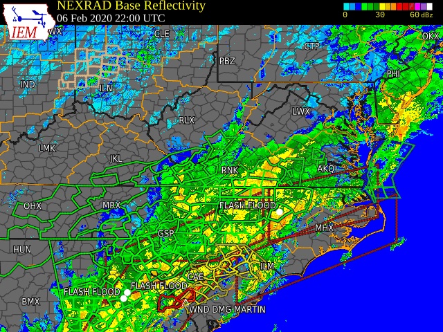
Fig. 1.15 Precipitation Resulting from Cold Air Damming East of the Appalachian Mountains

1.2.6.2.2. Tutorial Content

Coming Soon!

1.2.6.3. Sample Forecast #3: Southern Plains Winter Weather Event

1.2.6.3.1. Weather Summary

A polar vortex brought arctic air to much of the U.S. and Mexico. A series of cold fronts and vorticity disturbances helped keep this cold air in place for an extended period of time, resulting in record-breaking cold temperatures for many southern states and Mexico. This particular case captures two winter weather disturbances between February 14, 2021 at 06z and February 17, 2021 at 06z that brought several inches of snow to Oklahoma City. A lull on February 16, 2021 resulted in record daily low temperatures.

Weather Phenomena: Snow and record-breaking cold temperatures

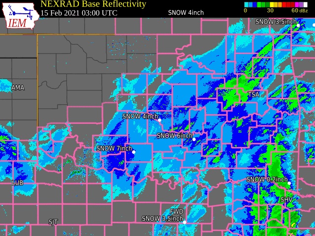
Fig. 1.16 Southern Plains Winter Weather Event Over Oklahoma City

1.2.6.3.2. Tutorial Content

Coming Soon!

1.2.6.4. Sample Forecast #4: Halloween Storm

1.2.6.4.1. Weather Summary

A line of severe storms brought strong winds, flash flooding, and tornadoes to the eastern half of the US.

Weather Phenomena: Flooding and high winds

• Storm Prediction Center (SPC) Storm Report for 20191031

Fig. 1.17 Halloween Storm 2019

1.2.6.4.2. Tutorial Content

Coming Soon!

1.2.6.5. Sample Forecast #5: Hurricane Barry

1.2.6.5.1. Weather Summary

Hurricane Barry made landfall in Louisiana on July 11, 2019 as a Category 1 hurricane. It produced widespread flooding in the region and had a peak wind speed of 72 mph and a minimum pressure of 992 hPa.

Weather Phenomena: Flooding, wind, and tornado reports

• Storm Prediction Center (SPC) Storm Report for 20190713

• Storm Prediction Center (SPC) Storm Report for 20190714

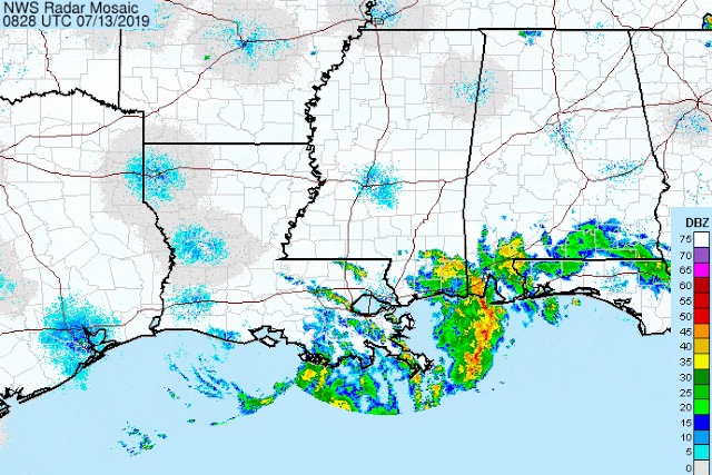
Fig. 1.18 Hurricane Barry Making Landfall

1.2.6.5.2. Tutorial Content

Coming Soon!