8. Limited Area Model (LAM) Grids: Predefined and User-Generated Options

In order to set up the workflow and generate an experiment with the SRW Application, the user must choose between four predefined FV3-LAM grids or generate a user-defined grid. At this time, full support will only be provided to those using one of the four predefined grids supported in the v2.0.0 release. However, preliminary information is provided at the end of this chapter that describes how users can leverage the SRW App workflow scripts to generate their own user-defined grid. Currently, this feature is not fully supported and is “use at your own risk.”

8.1. Predefined Grids

The SRW App v2.0.0 release includes four predefined limited area model (LAM) grids. To select a predefined grid, the PREDEF_GRID_NAME variable within the config.sh script must be set to one of the following four options:

• RRFS_CONUS_3km

• RRFS_CONUS_13km

• RRFS_CONUS_25km

• SUBCONUS_Ind_3km

These four options are provided for flexibility related to compute resources and supported physics options. The high-resolution 3-km CONUS grid generally requires more compute power and works well with three of the four supported physics suites (see Table 8.1). Low-resolution grids (i.e., 13-km and 25-km domains) require less compute power and should generally be used with the fourth supported physics suite: FV3_GFS_v16.

Table 8.1 Preferred grid and physics combinations for supported domains & physics suites

Grid	Physics Suite(s)
RRFS_CONUS_3km	FV3_RRFS_v1beta FV3_HRRR FV3_WoFS
SUBCONUS_Ind_3km	FV3_RRFS_v1beta FV3_HRRR FV3_WoFS
RRFS_CONUS_13km	FV3_GFS_v16
RRFS_CONUS_25km	FV3_GFS_v16

In theory, it is possible to run any of the supported physics suites with any of the predefined grids, but the results will be more accurate and meaningful with appropriate grid/physics pairings.

The predefined CONUS grids follow the naming convention (e.g., RRFS_CONUS_*km) of the prototype 3-km continental United States (CONUS) grid being tested for the Rapid Refresh Forecast System (RRFS). The RRFS will be a convection-allowing, hourly-cycled, FV3-LAM-based ensemble planned for operational implementation in 2024. All four supported grids were created to fit completely within the High Resolution Rapid Refresh (HRRR) domain to allow for use of HRRR data to initialize the SRW App.

8.1.1. Predefined 3-km CONUS Grid

The 3km CONUS domain is ideal for running the FV3_RRFS_v1beta physics suite, since this suite definition file (SDF) was specifically created for convection-allowing scales and is the precursor to the operational physics suite that will be used in the RRFS. The 3-km domain can also be used with the FV3_HRRR and FV3_WoFS physics suites, which likewise do not include convective parameterization. In fact, the FV3_WoFS physics suite is configured to run at 3-km or less and could therefore run with even higher-resolution user-defined domains if desired. However, the FV3_GFS_v16 suite generally should not be used with the 3-km domain because the cumulus physics used in that physics suite is not configured to run at the 3-km resolution.

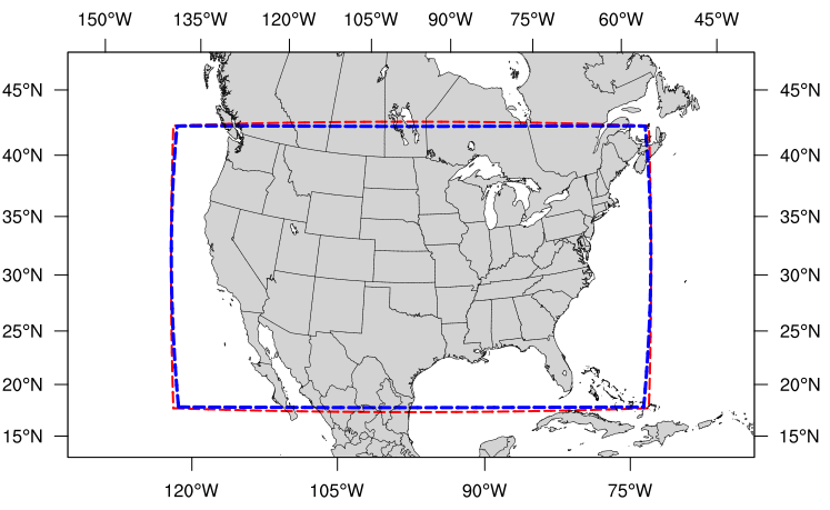
Fig. 8.1 The boundary of the RRFS_CONUS_3km computational grid (red) and corresponding write-component grid (blue).

The boundary of the RRFS_CONUS_3km domain is shown in Figure 8.1 (in red), and the boundary of the write-component grid sits just inside the computational domain (in blue). This extra grid is required because the post-processing utility (UPP) is unable to process data on the native FV3 gnomonic grid (in red). Therefore, model data are interpolated to a Lambert conformal grid (the write component grid) in order for UPP to read in and correctly process the data.

Note

While it is possible to initialize the FV3-LAM with coarser external model data when using the RRFS_CONUS_3km domain, it is generally advised to use external model data (such as HRRR or RAP data) that has a resolution similar to that of the native FV3-LAM (predefined) grid.

8.1.2. Predefined SUBCONUS Grid Over Indianapolis

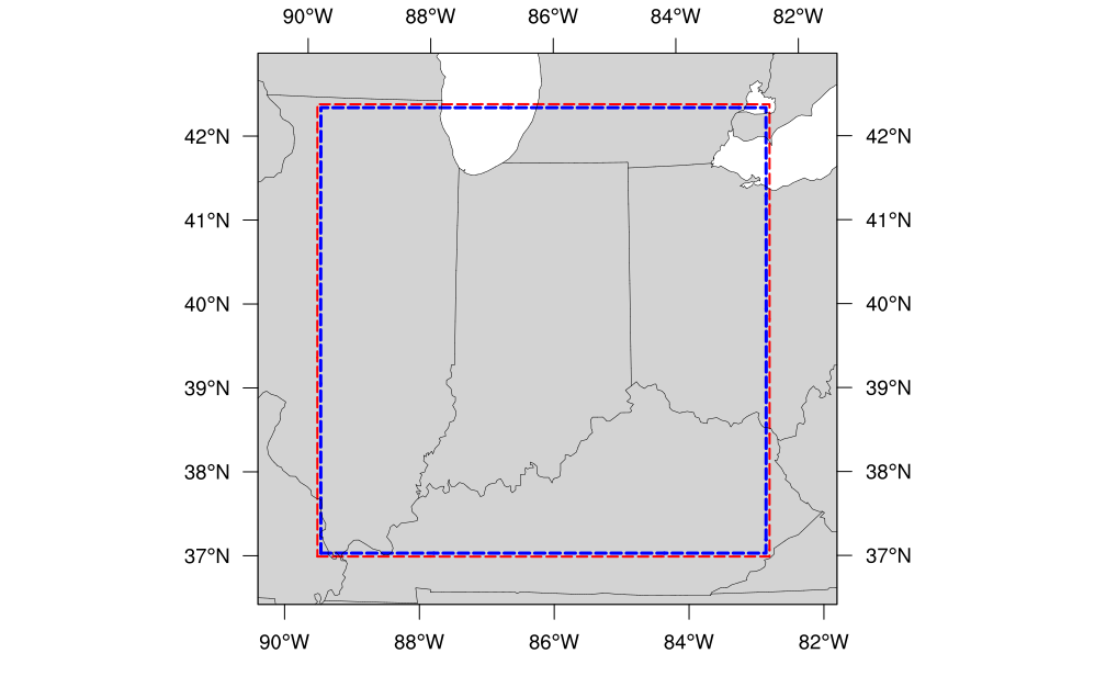
Fig. 8.2 The boundary of the SUBCONUS_Ind_3km computational grid (red) and corresponding write-component grid (blue).

The SUBCONUS_Ind_3km grid covers only a small section of the CONUS centered over Indianapolis. Like the RRFS_CONUS_3km grid, it is ideally paired with the FV3_RRFS_v1beta, FV3_HRRR, or FV3_WoFS physics suites, since these are all convection-allowing physics suites designed to work well on high-resolution grids.

8.1.3. Predefined 13-km Grid

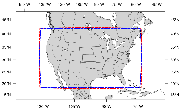
Fig. 8.3 The boundary of the RRFS_CONUS_13km computational grid (red) and corresponding write-component grid (blue).

The RRFS_CONUS_13km grid (Fig. 8.3) covers the full CONUS. This grid is meant to be run with the FV3_GFS_v16 physics suite. The FV3_GFS_v16 physics suite uses convective parameterizations, whereas the other supported suites do not. Convective parameterizations are necessary for low-resolution grids because convection occurs on scales smaller than 25km and 13km.

8.1.4. Predefined 25-km Grid

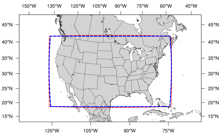
Fig. 8.4 The boundary of the RRFS_CONUS_25km computational grid (red) and corresponding write-component grid (blue).

The final predefined CONUS grid (Fig. 8.4) uses a 25-km resolution and is meant mostly for quick testing to ensure functionality prior to using a higher-resolution domain. However, for users who would like to use the 25-km domain for research, the FV3_GFS_v16 SDF is recommended for the reasons mentioned above.

Ultimately, the choice of grid is experiment-dependent and resource-dependent. For example, a user may wish to use the FV3_GFS_v16 physics suite, which uses cumulus physics that are not configured to run at the 3-km resolution. In this case, the 13-km or 25-km domain options are better suited to the experiment. Users will also have fewer computational constraints when running with the 13-km and 25-km domains, so depending on the resources available, certain grids may be better options than others.

8.2. Creating User-Generated Grids

While the four predefined grids available in this release are ideal for users just starting out with the SRW App, more advanced users may wish to create their own grid for testing over a different region and/or with a different resolution. Creating a user-defined grid requires knowledge of how the SRW App workflow functions. In particular, it is important to understand the set of scripts that handle the workflow and experiment generation (see Figure 4.2 and Figure 4.3). It is also important to note that user-defined grids are not a supported feature of the v2.0.0 release; however, information is being provided for the benefit of the FV3-LAM community.

With those caveats in mind, this section provides instructions for adding a new grid to the FV3-LAM workflow that will be generated using the “ESGgrid” method (i.e., using the regional_esg_grid code in the UFS_UTILS repository, where ESG stands for “Extended Schmidt Gnomonic”). We assume here that the grid to be generated covers a domain that (1) does not contain either of the poles and (2) does not cross the -180 deg –> +180 deg discontinuity in longitude near the international date line. Instructions for domains that do not have these restrictions will be provided in a future release.

The steps to add such a grid to the workflow are as follows:

1. Choose the name of the grid. For the purposes of this documentation, the grid will be called “NEW_GRID”.

2. Add NEW_GRID to the array valid_vals_PREDEF_GRID_NAME in the ufs-srweather-app/regional_workflow/ush/valid_param_vals.sh file.

3. In ufs-srweather-app/regional_workflow/ush/set_predef_grid_params.sh, add a stanza to the case statement case ${PREDEF_GRID_NAME} in for NEW_GRID. An example of such a stanza is given below along with comments describing the variables that need to be set.

To run a forecast experiment on NEW_GRID, start with a workflow configuration file for a successful experiment (e.g., config.sh, located in the ufs-srweather-app/regional_workflow/ush subdirectory), and change the line for PREDEF_GRID_NAME to the following:

PREDEF_GRID_NAME="NEW_GRID"

Then, generate a new experiment/workflow using the generate_FV3LAM_wflow.sh script in the usual way.

8.2.1. Code Example

The following is an example of a code stanza for “NEW_GRID” to be added to set_predef_grid_params.sh:

#
#---------------------------------------------------------------------
#
# Stanza for NEW_GRID.  This grid covers [provide a description of the
# domain that NEW_GRID covers, its grid cell size, etc].
#
#---------------------------------------------------------------------
#
"NEW_GRID")

# The method used to generate the grid.  This example is specifically
# for the "ESGgrid" method.

  GRID_GEN_METHOD= "ESGgrid"

# The longitude and latitude of the center of the grid, in degrees.

  ESGgrid_LON_CTR=-97.5
  ESGgrid_LAT_CTR=38.5

# The grid cell sizes in the x and y directions, where x and y are the
# native coordinates of any ESG grid. The units of x and y are in
# meters. These should be set to the nominal resolution we want the
# grid to have. The cells will have exactly these sizes in xy-space
# (computational space) but will have varying size in physical space.
# The advantage of the ESGgrid generation method over the GFDLgrid
# method is that an ESGgrid will have a much smaller variation in grid
# size in physical space than a GFDLgrid.

  ESGgrid_DELX="25000.0"
  ESGgrid_DELY="25000.0"

# The number of cells along the x and y axes.

  ESGgrid_NX=200
  ESGgrid_NY=112

# The width of the halo (in units of grid cells) that the temporary
# wide-halo grid created during the grid generation task (make_grid)
# will have. This wide-halo grid gets "shaved" down to obtain the
# 4-cell-wide halo and 3-cell-wide halo grids that the forecast model
# (as well as other codes) will actually use. Recall that the halo is
# needed to provide lateral boundary conditions to the forecast model.
# Usually, there is no need to modify this parameter.

  ESGgrid_WIDE_HALO_WIDTH=6

# The default physics time step that the forecast model will use. This
# is the (inverse) frequency with which (most of) the physics suite is
# called. The smaller the grid cell size is, the smaller this value
# needs to be in order to avoid numerical instabilities during the
# forecast. The values specified below are used only if DT_ATMOS is
# not explicitly set in the user-specified experiment configuration
# file config.sh. Note that this parameter may be suite dependent.

  if [ "${CCPP_PHYS_SUITE}" = "FV3_GFS_v16" ]; then
    DT_ATMOS=${DT_ATMOS:-"300"}
  elif [ "${CCPP_PHYS_SUITE}" = "FV3_RRFS_v1beta" ]; then
    DT_ATMOS=${DT_ATMOS:-"40"}
  else
    DT_ATMOS=${DT_ATMOS:-"40"}
  fi

# Default MPI task layout (decomposition) along the x and y directions and
# blocksize. The values specified below are used only if they are not explicitly
# set in the user-specified experiment configuration file config.sh.

  LAYOUT_X=${LAYOUT_X:-"5"}
  LAYOUT_Y=${LAYOUT_Y:-"2"}
  BLOCKSIZE=${BLOCKSIZE:-"40"}

# The parameters for the write-component (aka "quilting") grid. The
# Unified Post Processor (called by the ``RUN_POST_TN`` task) cannot
# process output on the native ESGgrid, so output fields are interpolated
# to a **write-component grid** before writing them to an output file.
# The output fields are not specified on the native grid
# but are instead remapped to this write-component grid. The variable
# "QUILTING", which specifies whether or not to use the
# write-component grid, is by default set to "TRUE".


  if [ "$QUILTING" = "TRUE" ]; then

# The number of "groups" of MPI tasks that may be running at any given
# time to write out the output. Each write group will be writing to
# one set of output files (a dynf${fhr}.nc and a phyf${fhr}.nc file,
# where $fhr is the forecast hour). Each write group contains
# WRTCMP_write_tasks_per_group tasks. Usually, it is sufficient to
# have just one write group. This may need to be increased if the
# forecast is proceeding so quickly that a single write group cannot
# complete writing to its set of files before there is a need/request
# to start writing the next set of files at the next output time (this
# can happen, for instance, if the forecast model is trying to write
# output at every time step).

    WRTCMP_write_groups="1"

# The number of MPI tasks to allocate to each write group.

    WRTCMP_write_tasks_per_group="2"

# The coordinate system for the write-component grid
# See the array valid_vals_WRTCMP_output_grid (defined in
# the script valid_param_vals.sh) for the values this can take on.
# The following example is specifically for the Lambert conformal
# coordinate system.

    WRTCMP_output_grid="lambert_conformal"

# The longitude and latitude of the center of the write-component
# grid.

    WRTCMP_cen_lon="${ESGgrid_LON_CTR}"
    WRTCMP_cen_lat="${ESGgrid_LAT_CTR}"

# The first and second standard latitudes needed for the Lambert
# conformal coordinate mapping.

    WRTCMP_stdlat1="${ESGgrid_LAT_CTR}"
    WRTCMP_stdlat2="${ESGgrid_LAT_CTR}"

# The number of grid points in the x and y directions of the
# write-component grid. Note that this xy coordinate system is that of
# the write-component grid (which in this case is Lambert conformal).
# Thus, it is in general different than the xy coordinate system of
# the native ESG grid.

    WRTCMP_nx="197"
    WRTCMP_ny="107"

# The longitude and latitude of the lower-left corner of the
# write-component grid, in degrees.

    WRTCMP_lon_lwr_left="-121.12455072"
    WRTCMP_lat_lwr_left="23.89394570"

# The grid cell sizes along the x and y directions of the
# write-component grid. Units depend on the coordinate system used by
# the grid (i.e., the value of WRTCMP_output_grid). For a Lambert
# conformal write-component grid, the units are in meters.

    WRTCMP_dx="${ESGgrid_DELX}"
    WRTCMP_dy="${ESGgrid_DELY}"

  fi
  ;;